Using example data: Cluster and match ensemble realizations

This notebook demonstrates how to use the RealizationClusterAndMatch plugin to combine ensemble forecast data from different sources, using clustering and matching techniques.

Aim: The goal is to reduce the number of ensemble members in a coarse-resolution forecast (primary input) by clustering similar realizations, and then match high-resolution ensemble members (secondary input) to these clusters. This approach enables the creation of a compact, representative set of ensemble forecasts that leverages both the broad coverage of global models and the spatial detail of regional models.

Why use clustering and matching?

Clustering helps identify representative patterns in large ensembles, reducing computational cost and simplifying interpretation. Matching allows high-resolution data to be mapped onto these clusters, improving local detail where available.

Hierarchy and precedence: This notebook uses a configurable hierarchy to control which data source is used for each forecast period. The hierarchy specifies:

• The primary input (e.g., a global or coarse-resolution ensemble) to be clustered.

• One or more secondary inputs (e.g., high-resolution ensembles) to be matched to clusters for selected forecast periods.

• For each forecast period, the hierarchy determines which model’s data takes precedence, allowing switching between sources depending on availability or user preference.

# Authors: The IMPROVER developers
# SPDX-License-Identifier: BSD-3-Clause

Check for required packages

This example requires the kmedoids package for clustering. Skip the example if it’s not available.

try:
    import kmedoids  # noqa: F401
except ImportError:
    raise RuntimeError("kmedoids package not available, skipping example")

Check for esmf_regrid availability

Check if esmf_regrid is available to determine the regridding method to use. If esmf_regrid is available, use area-weighted regridding for better accuracy. Otherwise, fall back to bilinear interpolation which is always available.

try:
    import esmf_regrid  # noqa: F401

    REGRID_MODE = "esmf-area-weighted"
except ImportError:
    REGRID_MODE = "bilinear"

Load example data

Load example coarse resolution data for clustering and visualization.

from iris.cube import CubeList

from improver import example_data_path
from improver.utilities.load import load_cube

# Get the path to the coarse resolution 6-hour forecast
data_path = example_data_path(
    "realization_cluster_and_match", "coarse_resolution_PT0006H00M.nc"
)

# Load the coarse resolution cube for visualization
coarse_cube_6h = load_cube(str(data_path))

print(coarse_cube_6h)

/home/docs/checkouts/readthedocs.org/user_builds/improver/conda/stable/lib/python3.13/site-packages/iris/common/mixin.py:212: FutureWarning: You are using legacy date precision for Iris units - max precision is seconds. In future, Iris will use microsecond precision - available since cf-units version 3.3 - which may affect core behaviour. To opt-in to the new behaviour, set `iris.FUTURE.date_microseconds = True`.
  warnings.warn(message, category=FutureWarning)
lwe_precipitation_rate / (m/s)      (realization: 18; projection_y_coordinate: 970; projection_x_coordinate: 1042)
    Dimension coordinates:
        realization                             x                            -                             -
        projection_y_coordinate                 -                            x                             -
        projection_x_coordinate                 -                            -                             x
    Scalar coordinates:
        forecast_period             21600 seconds
        forecast_reference_time     2025-12-01 06:00:00
        time                        2025-12-01 12:00:00
    Attributes:
        Conventions                 'CF-1.7'
        history                     '2025-12-01T10:36:00Z: StaGE Decoupler'
        institution                 'Met Office'
        mosg__model_configuration   'gl_ens'
        source                      'Met Office Unified Model'
        title                       'Post-Processed MOGREPS-G Forecast on UK 2 km Standard Grid'

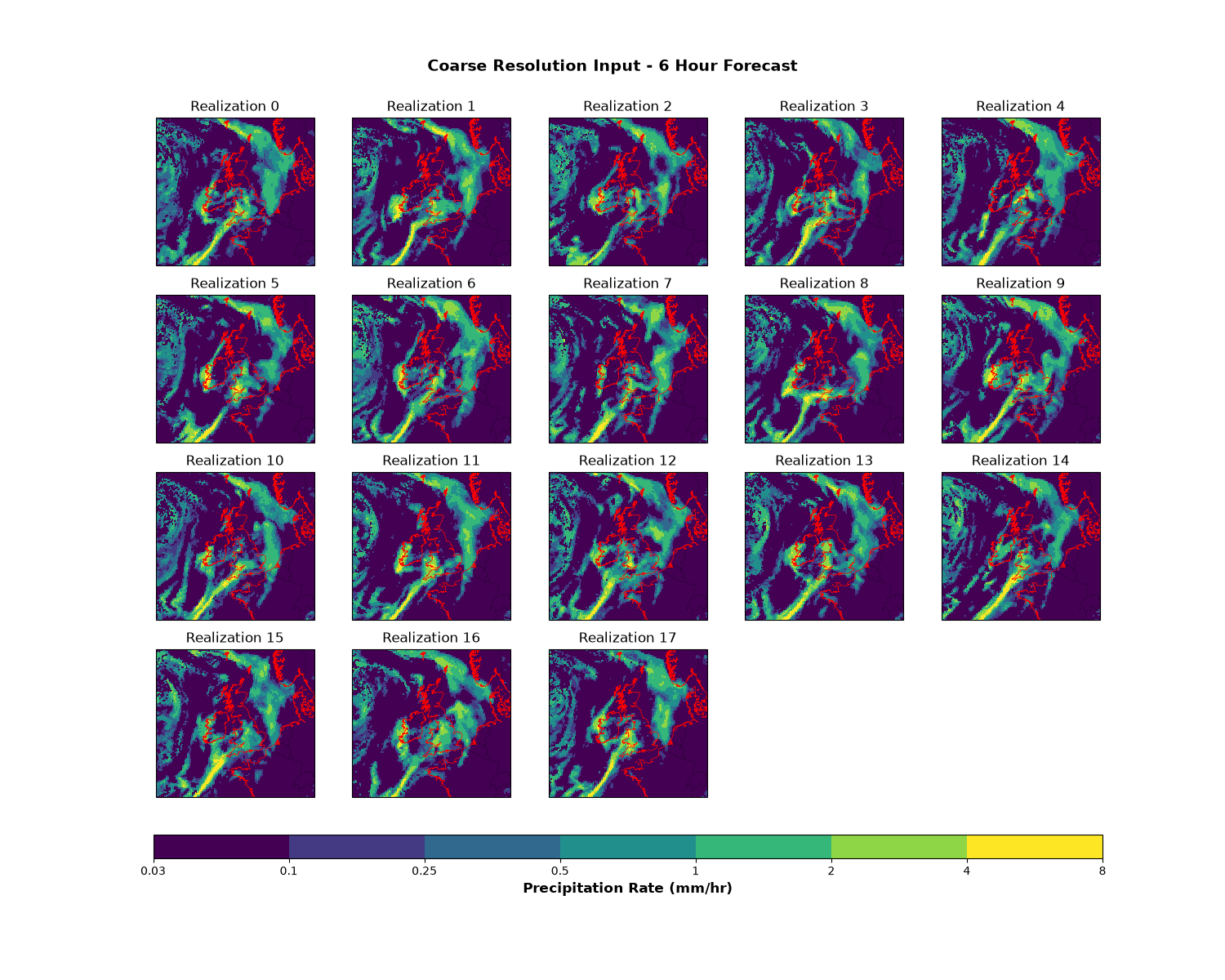
Visualize the input data

Plot all realizations from the coarse resolution 6-hour forecast. In this case, there is a broad eastward-moving front moving towards Norway, Denmark and Netherlands. There is narrower front in the south of the domain extending from south-west England in a southwestward direction. There is more scattered precipitation in the west of the domain.

import cartopy.feature as cfeature
import iris.plot as iplt
import matplotlib as mpl
import matplotlib.pyplot as plt

n_realizations = coarse_cube_6h.coord("realization").points.size

# Set up the color scale for precipitation (mm/hr)
precip_levels = [0.03, 0.1, 0.25, 0.5, 1, 2, 4, 8]
cmap = plt.cm.viridis
norm = mpl.colors.BoundaryNorm(precip_levels, cmap.N)

# Get the coordinate system from the cube
cube_crs = coarse_cube_6h.coord_system().as_cartopy_crs()

fig, axes = plt.subplots(4, 5, figsize=(15, 12), subplot_kw={"projection": cube_crs})
axes = axes.flatten()

for i in range(n_realizations):
    ax = axes[i]
    # Convert to mm/hr for plotting (original data in m/s)
    cube_plot = coarse_cube_6h[i].copy()
    cube_plot.data = cube_plot.data * 3600 * 1000  # m/s to mm/hr
    cube_plot.units = "mm/hr"

    mesh = iplt.pcolormesh(cube_plot, cmap=cmap, norm=norm, axes=ax)
    ax.coastlines(resolution="10m", linewidth=0.5, color="red")
    ax.add_feature(cfeature.BORDERS, linewidth=0.3, alpha=0.5)
    ax.set_title(f"Realization {i}")

# Hide unused subplots
for i in range(n_realizations, len(axes)):
    axes[i].axis("off")

# Add colorbar
cbar = plt.colorbar(
    mesh, ax=axes, orientation="horizontal", pad=0.05, fraction=0.05, aspect=40
)
cbar.set_label("Precipitation Rate (mm/hr)", fontsize=12, fontweight="bold")
cbar.set_ticks(precip_levels)
cbar.set_ticklabels([str(level) for level in precip_levels])

plt.suptitle(
    "Coarse Resolution Input - 6 Hour Forecast", fontsize=14, fontweight="bold", y=0.94
)
plt.show()

Load all input data

Load all forecast data files that will be used in the clustering and matching process.

# Load all data files
coarse_cube_12h = load_cube(
    str(
        example_data_path(
            "realization_cluster_and_match", "coarse_resolution_PT0012H00M.nc"
        )
    )
)
high_cube_6h = load_cube(
    str(
        example_data_path(
            "realization_cluster_and_match", "high_resolution_PT0006H00M.nc"
        )
    )
)
high_cube_12h = load_cube(
    str(
        example_data_path(
            "realization_cluster_and_match", "high_resolution_PT0012H00M.nc"
        )
    )
)
print("\nHigh resolution 6h:")
print(high_cube_6h)

High resolution 6h:
/home/docs/checkouts/readthedocs.org/user_builds/improver/conda/stable/lib/python3.13/site-packages/iris/common/mixin.py:212: FutureWarning: You are using legacy date precision for Iris units - max precision is seconds. In future, Iris will use microsecond precision - available since cf-units version 3.3 - which may affect core behaviour. To opt-in to the new behaviour, set `iris.FUTURE.date_microseconds = True`.
  warnings.warn(message, category=FutureWarning)
lwe_precipitation_rate / (m/s)      (realization: 3; projection_y_coordinate: 970; projection_x_coordinate: 1042)
    Dimension coordinates:
        realization                             x                           -                             -
        projection_y_coordinate                 -                           x                             -
        projection_x_coordinate                 -                           -                             x
    Scalar coordinates:
        forecast_period             21600 seconds
        forecast_reference_time     2025-12-01 06:00:00
        time                        2025-12-01 12:00:00
    Attributes:
        Conventions                 'CF-1.7'
        history                     '2025-12-01T07:53:52Z: StaGE Decoupler'
        institution                 'Met Office'
        mosg__model_configuration   'uk_ens'
        source                      'Met Office Unified Model'
        title                       'MOGREPS-UK Model Forecast on UK 2 km Standard Grid'

Create target grid for regridding

Create a coarser target grid that will be used for regridding during clustering. This grid is subsampled from the coarse resolution data to speed up clustering.

# Start with the coarse cube as a template
target_grid_cube = coarse_cube_6h[0].copy()

# Remove all attributes
target_grid_cube.attributes = {}

# Keep only x and y coordinates, remove all others
coords_to_keep = []
for coord in target_grid_cube.coords():
    if coord.name() in [
        target_grid_cube.coord(axis="x").name(),
        target_grid_cube.coord(axis="y").name(),
    ]:
        coords_to_keep.append(coord.name())

for coord in target_grid_cube.coords():
    if coord.name() not in coords_to_keep:
        target_grid_cube.remove_coord(coord)

# Rename the cube
target_grid_cube.rename("target_grid")

# Subsample: keep every 10th point along x and y axes
target_grid_cube = target_grid_cube[::10, ::10]

print("\nTarget grid cube:")
print(target_grid_cube)

Target grid cube:
target_grid / (m/s)                 (projection_y_coordinate: 97; projection_x_coordinate: 105)
    Dimension coordinates:
        projection_y_coordinate                             x                            -
        projection_x_coordinate                             -                            x

Step 1: Cluster the primary input

The first step is to cluster the primary (coarse resolution) input. This reduces the number of realizations by selecting representative members.

import iris
from iris import Constraint
from iris.util import equalise_attributes

from improver.clustering.realization_clustering import RealizationClusterAndMatch

# Combine all forecast periods from coarse resolution
primary_cube = coarse_cube_6h.copy()
primary_cubes = iris.cube.CubeList([coarse_cube_6h, coarse_cube_12h])
equalise_attributes(primary_cubes)
primary_cube = primary_cubes.merge_cube()
primary_cube.transpose([1, 0, 2, 3])

# Create the plugin instance
# Use esmf-area-weighted regridding if esmf_regrid is available,
# otherwise use bilinear interpolation
plugin = RealizationClusterAndMatch(
    hierarchy={"primary_input": "gl_ens", "secondary_inputs": {"uk_ens": [0, 6]}},
    model_id_attr="mosg__model_configuration",
    clustering_method="KMedoids",
    target_grid_name="target_grid",
    regrid_mode=REGRID_MODE,
    n_clusters=2,
)

# Cluster just the primary input to see the effect
clustered_primary, regridded_clustered_primary = plugin.cluster_primary_input(
    primary_cube, target_grid_cube
)

print("\nClustered primary cube:")
print(clustered_primary)

Clustered primary cube:
/home/docs/checkouts/readthedocs.org/user_builds/improver/conda/stable/lib/python3.13/site-packages/iris/common/mixin.py:212: FutureWarning: You are using legacy date precision for Iris units - max precision is seconds. In future, Iris will use microsecond precision - available since cf-units version 3.3 - which may affect core behaviour. To opt-in to the new behaviour, set `iris.FUTURE.date_microseconds = True`.
  warnings.warn(message, category=FutureWarning)
lwe_precipitation_rate / (m/s)                      (realization: 2; time: 2; projection_y_coordinate: 970; projection_x_coordinate: 1042)
    Dimension coordinates:
        realization                                             x        -                           -                             -
        time                                                    -        x                           -                             -
        projection_y_coordinate                                 -        -                           x                             -
        projection_x_coordinate                                 -        -                           -                             x
    Auxiliary coordinates:
        forecast_period                                         -        x                           -                             -
    Scalar coordinates:
        forecast_reference_time                     2025-12-01 06:00:00
    Attributes:
        Conventions                                 'CF-1.7'
        institution                                 'Met Office'
        mosg__model_configuration                   'gl_ens'
        primary_input_realization_to_cluster_medoid {0: 0, 1: 26}
        primary_input_realizations_to_clusters      {0: [0, 18, 19, 20, 21, 22, 23, 24, 25, 27, 28, 29, 30, 31, 32, 33, 34], 1: [26]}
        source                                      'Met Office Unified Model'
        title                                       'Post-Processed MOGREPS-G Forecast on UK 2 km Standard Grid'

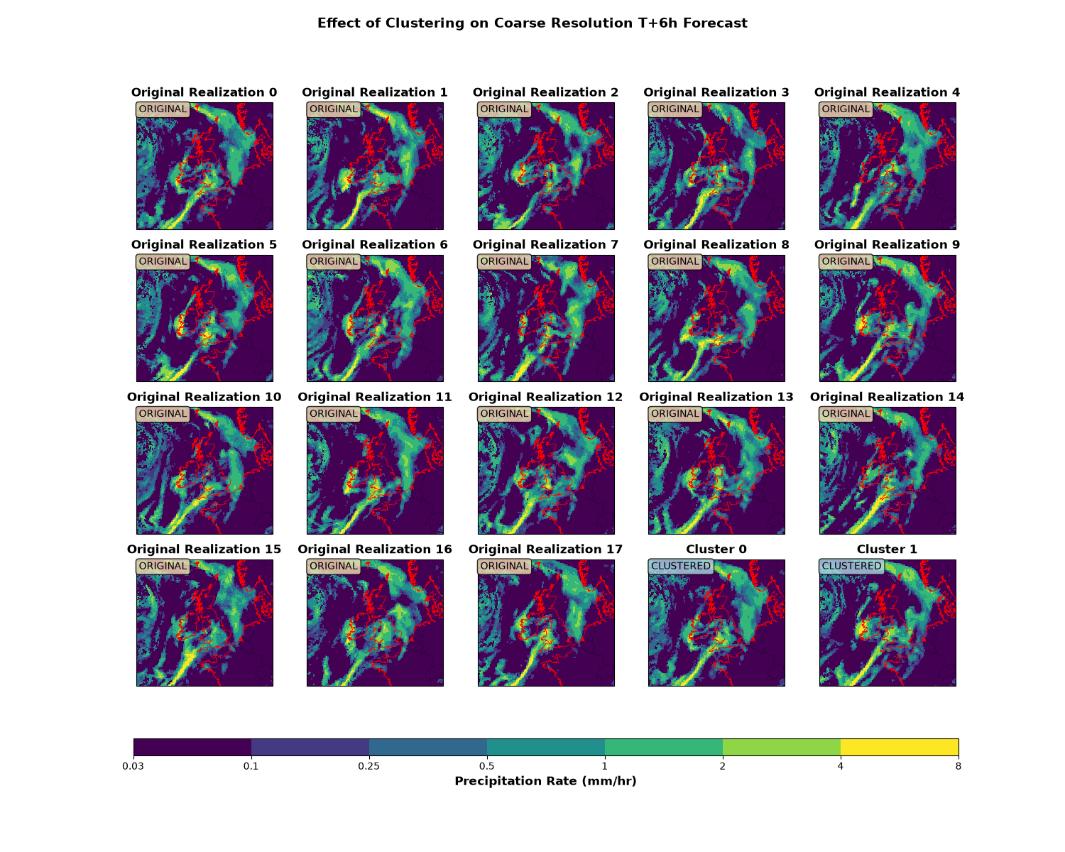
Visualize the clustering effect

Compare the original coarse resolution data with the clustered output. Clustering reduces the number of realizations while preserving key features. One source of difference between the realizations is the intensity of the precipitation in western Ireland, and this is one of the main differences between the two clusters.

n_clusters = clustered_primary.coord("realization").points.size

fig, axes = plt.subplots(4, 5, figsize=(15, 12), subplot_kw={"projection": cube_crs})
axes = axes.flatten()

# Plot original realizations (T+6h)
for i in range(n_realizations):
    ax = axes[i]
    # Convert to mm/hr for plotting
    cube_plot = coarse_cube_6h[i].copy()
    cube_plot.data = cube_plot.data * 3600 * 1000  # m/s to mm/hr
    cube_plot.units = "mm/hr"

    mesh = iplt.pcolormesh(cube_plot, cmap=cmap, norm=norm, axes=ax)
    ax.coastlines(resolution="10m", linewidth=0.5, color="red")
    ax.add_feature(cfeature.BORDERS, linewidth=0.3, alpha=0.5)
    ax.set_title(f"Original Realization {i}", fontweight="bold")
    ax.text(
        0.02,
        0.98,
        "ORIGINAL",
        transform=ax.transAxes,
        fontsize=10,
        verticalalignment="top",
        bbox=dict(boxstyle="round", facecolor="wheat", alpha=0.8),
    )

# Plot clustered output (extract T+6h)
fp_6h = 6 * 3600  # 6 hours in seconds
clustered_6h = clustered_primary.extract(Constraint(forecast_period=fp_6h))
for i in range(n_clusters):
    ax = axes[n_realizations + i]
    # Convert to mm/hr for plotting
    cube_plot = clustered_6h[i].copy()
    cube_plot.data = cube_plot.data * 3600 * 1000  # m/s to mm/hr
    cube_plot.units = "mm/hr"

    mesh = iplt.pcolormesh(cube_plot, cmap=cmap, norm=norm, axes=ax)
    ax.coastlines(resolution="10m", linewidth=0.5, color="red")
    ax.add_feature(cfeature.BORDERS, linewidth=0.3, alpha=0.5)
    ax.set_title(f"Cluster {i}", fontweight="bold")
    ax.text(
        0.02,
        0.98,
        "CLUSTERED",
        transform=ax.transAxes,
        fontsize=10,
        verticalalignment="top",
        bbox=dict(boxstyle="round", facecolor="lightblue", alpha=0.8),
    )

# Hide unused subplots
for i in range(n_realizations + n_clusters, len(axes)):
    axes[i].axis("off")

# Add colorbar
cbar = plt.colorbar(
    mesh, ax=axes, orientation="horizontal", pad=0.08, fraction=0.03, aspect=50
)
cbar.set_label("Precipitation Rate (mm/hr)", fontsize=12, fontweight="bold")
cbar.set_ticks(precip_levels)
cbar.set_ticklabels([str(level) for level in precip_levels])

plt.suptitle(
    "Effect of Clustering on Coarse Resolution T+6h Forecast",
    fontsize=14,
    fontweight="bold",
)
plt.show()

Step 2: Perform full clustering and matching

Now apply the full plugin to cluster the primary input and match secondary inputs to the clusters. The hierarchy specifies that:

• gl_ens (global/coarse ensemble) is the primary input to be clustered

• uk_ens (UK/high resolution ensemble) is a secondary input that will be matched to the clusters for forecast periods 0-6 hours

# Combine into a CubeList
cubes = CubeList(
    [coarse_cube_6h, coarse_cube_12h, high_cube_6h, high_cube_12h, target_grid_cube]
)

# Apply clustering and matching
result_cube = plugin(cubes)

print("\nFinal result cube:")
print(result_cube)

Final result cube:
/home/docs/checkouts/readthedocs.org/user_builds/improver/conda/stable/lib/python3.13/site-packages/iris/common/mixin.py:212: FutureWarning: You are using legacy date precision for Iris units - max precision is seconds. In future, Iris will use microsecond precision - available since cf-units version 3.3 - which may affect core behaviour. To opt-in to the new behaviour, set `iris.FUTURE.date_microseconds = True`.
  warnings.warn(message, category=FutureWarning)
lwe_precipitation_rate / (m/s)                      (time: 2; realization: 2; projection_y_coordinate: 970; projection_x_coordinate: 1042)
    Dimension coordinates:
        time                                             x               -                           -                             -
        realization                                      -               x                           -                             -
        projection_y_coordinate                          -               -                           x                             -
        projection_x_coordinate                          -               -                           -                             x
    Auxiliary coordinates:
        forecast_period                                  x               -                           -                             -
    Scalar coordinates:
        forecast_reference_time                     2025-12-01 06:00:00
    Attributes:
        Conventions                                 'CF-1.7'
        cluster_sources                             '{"0": {"gl_ens": [43200], "uk_ens": [21600]}, "1": {"gl_ens": [43200], ...'
        institution                                 'Met Office'
        primary_input_realization_to_cluster_medoid '{"0": 0, "1": 9}'
        primary_input_realizations_to_clusters      '{"0": [0, 1, 2, 3, 4, 5, 6, 7, 8, 10, 11, 12, 13, 14, 15, 16, 17], "1": ...'
        secondary_input_realizations_to_clusters    '{"uk_ens": {"0": [{"realization": 3, "forecast_periods": [21600]}], "1": ...'
        source                                      'Met Office Unified Model'

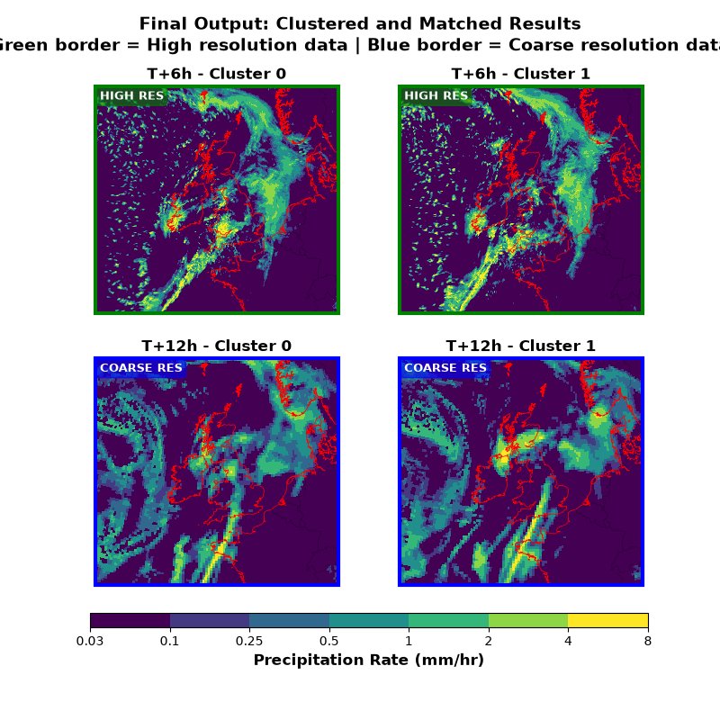
Visualize the results - highlighting data sources

Plot the clustered and matched output for each forecast period. The hierarchy specified that uk_ens (high resolution) should be used for forecast periods 0-6 hours, so: - T+6h uses HIGH RESOLUTION data (uk_ens matched to clusters) - T+12h uses COARSE RESOLUTION data (gl_ens clustered primary input) At T+6h, one of the main differences between the clusters is the extent of the precipitation over the sea to the north and west of Cornwall.

forecast_periods = result_cube.coord("forecast_period").points
n_periods = len(forecast_periods)
n_clusters = result_cube.coord("realization").points.size

fig, axes = plt.subplots(2, 2, figsize=(8, 8), subplot_kw={"projection": cube_crs})
axes = axes.flatten()

plot_idx = 0
for period_idx, fp in enumerate(forecast_periods):
    fp_cube = result_cube.extract(Constraint(forecast_period=fp))
    fp_hours = fp / 3600  # Convert seconds to hours

    # Determine data source based on forecast period
    # hierarchy specified uk_ens for [0, 6] hours
    if fp_hours <= 6:
        source = "HIGH RES"
        full_source = "HIGH RESOLUTION (uk_ens)"
        color = "green"
    else:
        source = "COARSE RES"
        full_source = "COARSE RESOLUTION (gl_ens)"
        color = "blue"

    for cluster_idx in range(n_clusters):
        ax = axes[plot_idx]
        plot_idx += 1

        # Convert to mm/hr for plotting
        cube_plot = fp_cube[cluster_idx].copy()
        cube_plot.data = cube_plot.data * 3600 * 1000  # m/s to mm/hr
        cube_plot.units = "mm/hr"

        mesh = iplt.pcolormesh(cube_plot, cmap=cmap, norm=norm, axes=ax)
        ax.coastlines(resolution="10m", linewidth=0.5, color="red")
        ax.add_feature(cfeature.BORDERS, linewidth=0.3, alpha=0.5)
        ax.set_title(f"T+{int(fp_hours)}h - Cluster {cluster_idx}", fontweight="bold")

        # Add data source label
        ax.text(
            0.02,
            0.98,
            source,
            transform=ax.transAxes,
            fontsize=9,
            verticalalignment="top",
            bbox=dict(boxstyle="round", facecolor=color, alpha=0.6, edgecolor=color),
            color="white",
            fontweight="bold",
        )

        # Add colored border to indicate data source
        for spine in ax.spines.values():
            spine.set_edgecolor(color)
            spine.set_linewidth(3)

# Add colorbar below the subplots
cbar = plt.colorbar(
    mesh, ax=axes, orientation="horizontal", pad=0.05, fraction=0.05, aspect=40
)
cbar.set_label("Precipitation Rate (mm/hr)", fontsize=12, fontweight="bold")
cbar.set_ticks(precip_levels)
cbar.set_ticklabels([str(level) for level in precip_levels])

plt.suptitle(
    "Final Output: Clustered and Matched Results\n"
    "Green border = High resolution data | Blue border = Coarse resolution data",
    fontsize=14,
    fontweight="bold",
)
plt.show()

Summary of the process

Clustering and Matching Summary

Input (coarse resolution): 18 realizations

Output (clustered): 2 clusters

Number of forecast periods: 2

Data source by forecast period:

• T+ 6h: HIGH RESOLUTION (uk_ens) - matched to clusters

• T+12h: COARSE RESOLUTION (gl_ens) - primary clustered input

What happened:

1. The coarse resolution (gl_ens) ensemble was clustered using KMedoids to reduce 18 realizations to 2 representative clusters

2. For T+6h: High resolution (uk_ens) realizations were matched to these clusters based on mean squared error, providing higher resolution output

3. For T+12h: The clustered coarse resolution data was used directly (no high resolution data available for this period in the hierarchy)